Reinforcement Learning with Q-Learning

Reinforcement learning is a type of machine learning that does not require a dataset to learn from. It can learn from the experience it gathers. Let’s think of the network as of an agent in a defined environment. The agent learns about the environment through the actions it performs and a feedback it receives. For each action, it will receive a reward, if the action was good or a penalty otherwise. Based on the knowledge the agent has gathered and the current state of the environment, the next action is chosen.

Q-Learning

Q-Learning is a a value-based technique of the reinforcement learning. The job of the network is to tell the agent what action should it perform in each step based on the environment state and the knowledge it has. It finds a policy to make the most optimal actions to achieve the goal.

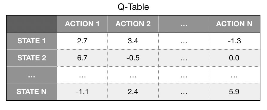
Q-Learning is using a table, called Q-Table, to keep the best score for each possible action in each state and updates it after each step. The process starts without any data, so the table should be populated with a default value. Because of that, the agent has to randomly choose an action at the beginning. It is very similar to people behavior. If we do not know what to choose, we will randomly select one option and see and learn from the result. That’s exactly how Q-Learning works.

How many decisions will be made based on the knowledge and how many of them will just be randomly selected is configurable. It is highly advised to change the proportion dynamically along with increasing the experience of the agent. Yet another reference to people. The more experienced we are, the more decisions we make based on our knowledge instead of relying on fate.

Q-table allows us to simply read the best action to perform for current state of the environment. Updating values in the table is based on the algorithm called a Q-Function.

Algorithm

As a first step, we initialize the Q-Table with fixed values, defined by us. Then, for each action A in state S, we will receive a reward R and a new state S’. All the data is passed to  the Q-Function to update the Q-Table with a new Q-Value. Q-Function simply updates value in the table in iterations based on old value and the new data.

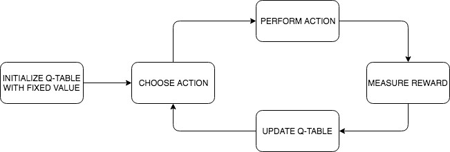
Q-Function calculates a new Q-Value based on the old value and 3 parameters. Q-Value or Q(S,A) stands for the quality of taking action A in state S. Developers have to select values for the parameters. They can be either constant or be adjusted dynamically along with growing knowledge of the agent. After each step, the model is updated according to the formula below.

Q(s,a): =Q(s,a)+alpha*[reward+gamma*maxQ(s’,a’)-Q(s,a)

Parameter alpha (range from 0 to 1) is called a learning rate and it defines to what extent new information is used. If we set this parameter to 0, the network will not learn at all.

Reward parameter determines the value received for changing the state from state s to s’ with action a. As mentioned before, it can be a penalty, in case a performed action does not improve the total score and does not move us closer to the goal.

Parameter gamma (range from 0 to 1) is a discount factor which defines the importance of future profits compared to current ones. Towards long-term profits, the gamma parameter should be set closer to the maximum value.

Example

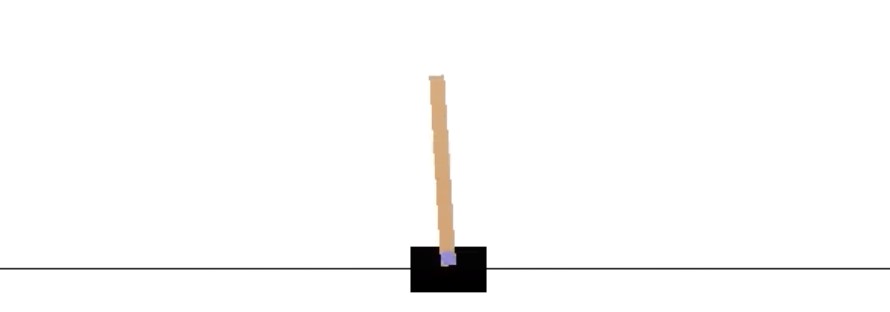
CartPole-v1 from Gym OpenAI environments is a good example to see reinforcement learning in action. We have a pendulum that is mounted to a moving block. The block can move to either left or right and the goal is to balance the pendulum and prevent it from falling over. More details here

First, we need to discretize the state parameters. Considering each angle and each inch is too complex. We do not need to know the exact position of the block and the pole. An approximation will be enough. The total range of position is divided into buckets. The more buckets we have, the more time will be required to learn the agent. We need to find the optimum quantity.

Two parameters related with the block do not contribute too much, so we omit them. We focus only on the angle and the angular velocity of the pole. CartPole has some boundaries for each parameter, that are declared below with a few constants that will be used in the code. I select to discretize both the angle and the angular velocity to 12 buckets.

State of the environment consists of 4 values corresponding to 4 parameters. For the first two of them we will return 0 and for the rest, we will return a bucket number appropriate to the received value.

import math
import gym

ENV = gym.make('CartPole-v1')

ANGLE_BUCKETS = 12
ANGLE_LOWER_BOUND = ENV.observation_space.low[2]
ANGLE_UPPER_BOUND = ENV.observation_space.high[2]
ANGLE_RANGE = ANGLE_UPPER_BOUND - ANGLE_LOWER_BOUND
ANGLE_INTERVAL = ANGLE_RANGE / float(ANGLE_BUCKETS)

ANGULAR_VELOCITY_BUCKETS = 12
ANGULAR_VELOCITY_LOWER_BOUND = -math.radians(50)
ANGULAR_VELOCITY_UPPER_BOUND = math.radians(50)
ANGULAR_VELOCITY_RANGE = ANGULAR_VELOCITY_UPPER_BOUND - ANGULAR_VELOCITY_LOWER_BOUND
ANGULAR_VELOCITY_INTERVAL = ANGULAR_VELOCITY_RANGE / float(ANGULAR_VELOCITY_BUCKETS)

State of the environment consists of 4 values corresponding to 4 parameters. For the first two of them we will return 0 and for the rest, we will return a bucket number appropriate to the received value.

def discretise(state):
    angle = discretise_angle(state[2])
    angular_velocity = discretise_angular_velocity(state[3])
    return 0, 0, angle, angular_velocity

def discretise_angle(value):
    return get_bucket_number(value, ANGLE_BUCKETS, ANGLE_LOWER_BOUND, ANGLE_INTERVAL)

def discretise_angular_velocity(value):
    return get_bucket_number(value, ANGULAR_VELOCITY_BUCKETS, 
        ANGULAR_VELOCITY_LOWER_BOUND, ANGULAR_VELOCITY_INTERVAL)

def get_bucket_number(value, buckets, lower_bound, interval):
    for i in range(1, buckets):
        tmp = lower_bound + (i * interval)
        if value < tmp:
            return i
        i += 1
    return buckets

The decision about the action is based on the Q-Table, which keep Q-Values for each state and action. If the is no record in the table, we randomly choose an action. Epsilon parameter defines a trade-off between exploration and exploitation, whether to make a random move or to base on the Q-Table. We start with a high value and decrease it along with subsequent attempts.

import random

MAX_ATTEMPTS = 10000

def calculate_epsilon(attempt):
    progress = attempt / float(MAX_ATTEMPTS)
    if progress < 0.15: return 0.9
    if progress < 0.55: return 0.7
    if progress < 0.85: return 0.4
    return 0.1

def pick_action(state, attempt):
    if state in Q_TABLE and random.random() > calculate_epsilon(attempt):
        return pick_best_action(state)
    return ENV.action_space.sample()

def pick_best_action(state):
    return 0 if Q_TABLE[state][0] > Q_TABLE[state][1] else 1

Finally, we can merge everything together and see the code in action. When variable done is positive, it means the game is over and we lost. Now, we can try different configurations and see if the result gets any better.

for attempt in range(MAX_ATTEMPTS):
    total_reward = 0.0
    done = False
    state = discretise(ENV.reset())

    while not done:
        ENV.render()
        action = pick_action(state, attempt)
        new_state, reward, done, info = ENV.step(action)
        new_state = discretise(new_state)
        update_knowledge(action, state, new_state, reward, attempt)
        state = new_state
        total_reward += reward

    print(total_reward)